Projection onto the L1-Norm Ball

In this post we will discuss a frequently visited problem in convex optimization: projection onto the $\ell_1$-norm ball. I think this is a great example to understand the concepts of duality and piecewise functions and the phenomenon called sparsity, where the solution to a problem contains mostly zeros, and only some remain “activated.”

The Problem

Suppose we have a vector $a \in \mathbb{R}^n$ and want to find another vector $x$ in an $\ell_1$-norm ball such that the distance between $a$ and $x$ is the smallest possible. In other words, we seek to solve the following problem

The constraint $\lVert x \rVert_1 \leq \kappa$ denotes the $\ell_1$-norm ball of radius $\kappa > 0$ (that is, all the points whose $\ell_1$ norm is at most $\kappa$) and $f(x)$ is the primal objective function.

Does this problem have a closed-form solution? Yes, but not always. Like all projection problems, if $a$ is already in the convex set ($\lVert a \rVert_1 \leq \kappa$) then the solution is simply $x = a$, and we are done. Otherwise, we will need to approximate the solution.

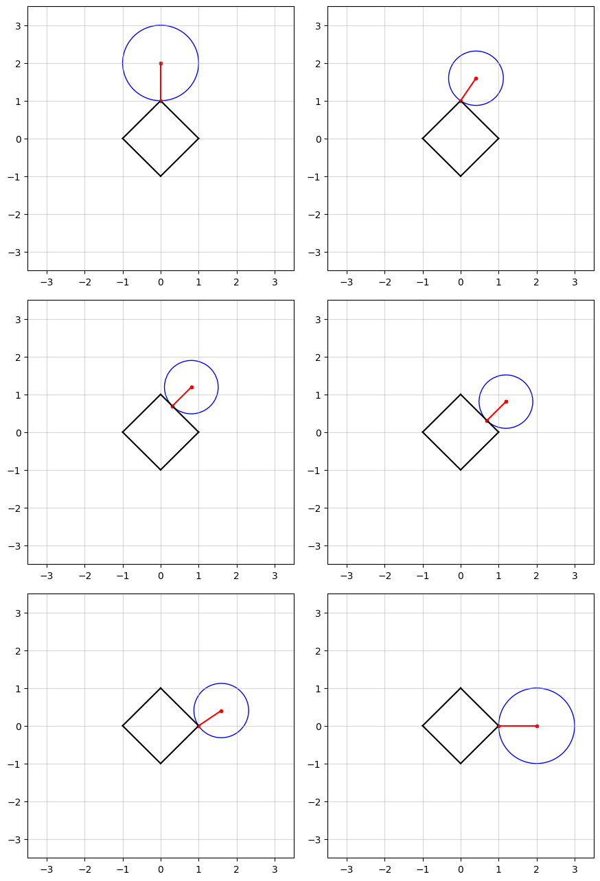
In the above figure, we see an example in $n=2$ dimensions. The black square (containing all points on and within its boundaries) represents the $\ell_1$-norm ball of radius $\kappa = 1$. The center of the blue circle, in red, is the vector $a$ and the radius of the circle is the smallest distance from $a$ to the $\ell_1$-norm ball.

Duality

It is easy to see that $\eqref{eq:primal}$ is a convex optimization problem as its objective and constraint are both convex. Note that in this case, $x = 0$ is a strictly feasible solution, which means, by Slater’s condition, strong duality holds. We therefore will aim to solve $\eqref{eq:primal}$ by maximizing its dual function. Let $\gamma \geq 0$ be the dual variable; the Lagragian is

Finding the dual objective function requires us to minimize $L(x, \gamma)$ with respect to $x$. Notice that we can rewrite the Lagrangian as

where the subscript $i$ denotes the $i$th element of a vector. If we let

then minimizing $L(x, \gamma)$ with respect to $x$ means to minimize each $s_i(x_i, \gamma)$ with respect to $x_i$. Fortunately, the problem $\min_{x_i} s_i(x_i, \gamma)$ has a unique and closed-form solution:

This is is called the soft thresholding operator for $\gamma$. Equation $\eqref{eq:threshold_si}$ shows us how to convert a dual solution $\gamma$ to a primal solution $x$. Now, if we let $s_i^*(\gamma) = \min_{x_i} s_i(x_i, \gamma) = s_i(x_i(\gamma), \gamma)$, the dual objective is

We know that $g$ is a concave function by design. Furthermore, since the solution to $\min_{x_i} s_i(x_i, \gamma)$ is unique for every $\gamma \geq 0$, by Danskin’s theorem, each $s_i^*$ is differentiable, which makes $g$ differentiable as well. We can easily verify that the derivative of $g$ is

So far we have been able to find the dual function $g(\gamma)$ and its derivative $g’(\gamma)$. Now we will explore a method to maximize $g(\gamma)$ and recover the primal optimal solution.

Optimizing the Dual Function

As a reminder, we will aim to solve the problem

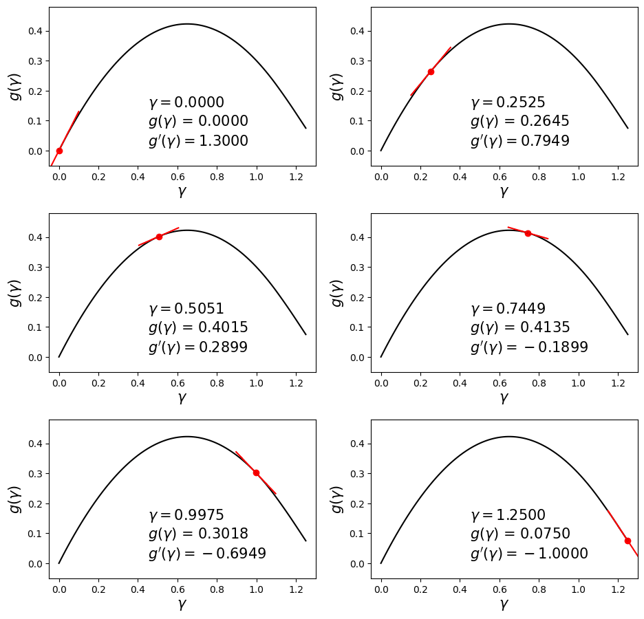
Since $g$ is concave and differentiable, we can aim to maximize it by using a hill-climbing algorithm such as gradient ascent with backtracking line search. Below is an example dual function and its derivative at various values of $\gamma$.

In this post we will solve this problem using a different method called bisection. The aim here is to set the derivative to zero and solve for $\gamma$. In other words, we seek the solution to $g’(\gamma) = 0$. The bisection method requires us to have a range $[\gamma_{\min}, \gamma_{\max}]$ in which we are sure the optimal solution $\gamma^*$ lies.

First, since $\gamma^*$ must be feasible, we set $\gamma_{\min} = 0$. To find an upper bound, note that since the optimal objective value for Problem $\eqref{eq:primal}$ must be non-negative, and strong duality holds, the optimal value for Problem $\eqref{eq:dual}$ is also non-negative. This implies that

Therefore,

where the second inequality is due to the fact that \(x_i(\gamma^*)\) is the minimizer if $s_i(x, \gamma^*)$. So an upper bound we can set for \(\gamma^*\) is \(\gamma_{\max} = \frac{1}{2 \kappa} \lVert a \rVert_2^2\).

Now that we know \(\gamma^*\) is in between $\gamma_{\min} = 0$ and \(\gamma_{\max} = \frac{1}{2 \kappa} \lVert a \rVert_2^2\), the bisection method works as follows. First, let $\gamma = (\gamma_{\min} + \gamma_{\max}) / 2$. If the sign of $g’(\gamma)$ is the same as that of $g’(\gamma_{\min})$, then $\gamma_{\min}$ is updated to $\gamma$. Otherwise, $\gamma_{\max}$ is updated to $\gamma$. It is simple as that! The method is also guaranteed to converge, as after each iteration, the length of the interval $[\gamma_{\min}, \gamma_{\max}]$ is reduced by half.

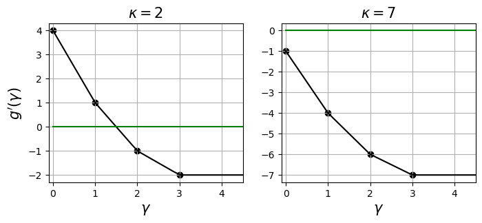
Another point to note is that \(g'\) is a monotonically non-increasing function. It achieves a minimum of \(-\kappa\) when \(\gamma \geq \max_i \left\{ \lvert x_i \rvert \right\}\) and a maximum of \(-\kappa + \lVert a \rVert_1\) when \(\gamma \leq \min_i \left\{ \lvert x_i \rvert \right\}\). When \(\lVert a \lVert \leq \kappa\), $g’$ is always negative so the solution can be incorrect. In this special case, we can directly conclude the solution $x = a$ without having to solve anything else.

The figures above show the derivative of a dual function where $a = [1,2,3]^\top$. The dark green horizontal line depicts $y = 0$. We can see that $g’$ is non-increasing and piecewise. In the left plot, $\kappa$ is set to $2 < \lVert a \rVert_1 = 6$, which allows $g’$ to cross the $y = 0$ line and so the solution to $g’(\gamma)$ exists. On the other hand, in the right plot where $\kappa$ exceeds $\lVert a \rVert_1$, no solution exists. In this case one can output $a$ as the solution already.

Implementation

Here is a simple Python implementation of the bisection method for maximizing the dual objective. First we define a few functions.

def primal_fn(x, a):
    return 0.5 * np.sum((x - a) ** 2)

# Vectorize the computation of s_i(x, gamma)
def s(x, gamma, a):
    return 0.5 * (x - a) ** 2 + gamma * np.abs(x)

def x_gamma(gamma, a):
    sol = np.zeros_like(a)
    idx = a > gamma
    sol[idx] = a[idx] - gamma
    idx = a < - gamma
    sol[idx] = a[idx] + gamma
    return sol

def dual_fn(gamma, kappa, a):
    x = x_gamma(gamma, a)
    return - kappa * gamma + np.sum(s(x, gamma, a))

def dual_grad(gamma, kappa, a):
    return - kappa + np.sum(np.maximum(np.abs(a) - gamma, 0))

Then, the bisection method is straightforward. We can let the iterations run until the difference $\gamma_{\max} - \gamma_{\min}$ reaches below a pre-defined error $\varepsilon$, at which point the derivative should be close enough to $0$.

def bisection(a, kappa, eps=1e-5):
    gamma_min, gamma_max = 0, (1 / (2 * kappa)) * np.sum(a ** 2)
    # Run until gamma_max and gamma_min are the same
    while gamma_max - gamma_min > eps:
        gamma = (gamma_max + gamma_min) / 2
        grad = dual_grad(gamma, kappa, a)
        if grad < 0: 
            gamma_max = gamma
        else:
            gamma_min = gamma
    return gamma

The first two plots in this post are produced using the following code.

# Point to be projected
a = np.array([1.1, 1.2])
# Radius of the ell_1 norm ball
kappa = 1
# Find approximate solution to the dual problem
dual_solution = bisection(a, kappa, eps=1e-5)
# Convert to the primal solution
primal_solution = x_gamma(dual_solution, a)

Sparseness of the Solution

In the figure at the top of this post, you probably have observed that as $a$ moves, there seems to be a “region” of $a$ in which the solution stays in a vertex of the square. Projection onto the $\ell_1$-norm ball has an interesting characteristic: in high dimensions, the optimal solution has a tendency to be sparse, which means most of its elements are driven to zero. To see how, let’s try an example.

>>> np.random.seed(100)
>>> a = np.random.randn(100)
>>> dual_solution = bisection(a, kappa=1, eps=1e-10)
>>> primal_solution = x_gamma(dual_solution, a)
>>> print(np.count_nonzero(primal_solution))
5

In this example, I generated a $100$-dimensional vector $a$ by independently sampling $100$ samples from the standard normal distribution. After projection, the solution only contains $5$ non-zero values. Only $5$ out of $100$ elements remain non-zero! (Be careful: I set $\varepsilon$ to be very small but it’s probably better to check equality using np.allclose to compare two floating point numbers.)

You may ask, “What’s the significance of this?” The tendency to drive most variables to zero is behind the success of the lasso method. Imagine you are performing a regression analysis with many, many variables. The lasso, or $\ell_1$ regularized, problem is

where $X$ is the design matrix, $y$ is the ground-truth labels and $\lambda$ is the regularization strength. Note that the formulation of lasso regression is not exactly the problem discussed in this method: the variable has to go through a linear transformation in lasso. However, observations remain similar: the solution $w^*$ to this problem tends to be sparse where most weights are driven to zero.

While $\ell_2$ is a more popular regularizer, $\ell_1$ may be preferred if you like to assess features’ importance: those with non-zero coefficients tend to be very few and represent the most important features you may want to keep during feature selection.

Conclusion

In this post we explore the problem of projection onto an $\ell_1$-norm ball. We formalize the primal problem and see how the dual problem can be expressed and optimized. We also observe that the solution tends to be sparse in high dimensions.

Several things deserve some mentioning in these concluding remarks. First, we have yet to talk about the asymptotic complexity of solving $\ell_1$ projection. That is, given some tolerance $\epsilon$, how much time do we need to achieve an approximate solution $x$ to Problem $\eqref{eq:primal}$ such that $f(x) - f(x^*) < \epsilon$? Second, you may be interested in a variant of $\ell_1$ projection called simplex projection, where the variable $x$ is also constrained to be non-negative. In this case the Lagrangian in $\eqref{eq:lagrangian}$ must involve another set of variables for the constraints $x_i \geq 0, i = 1, \ldots, n$, and a different optimization algorithm is needed. Third, minimizing the lasso objective as in $\eqref{eq:lasso}$ deserves some discussion, too. The resources below should offer some answer to these questions.

Resources

1. Ryan Tibshirani’s lectures on convex optimization, specifically those on duality and proximal gradient descent.
2. Convex Optimization by Boyd and Vandenberghe.
3. Efficient Projections onto the $\ell_1$-Ball for Learning in High Dimensions by John Duchi, Shai Shalev-Shwartz, Yoram Singer and Tushar Chandra.